Welcome to HI-FRIENDS SDC2’s documentation!¶

The SKA Data Challenge 2¶

These pages contain the documentation related to the software developed by the HI-FRIENDS team to analyse SKA simulated data to participate in the second SKA Science Data Challenge (SDC2). The SDC2 is a source finding and source characterisation data challenge to find and characterise the neutral hydrogen content of galaxies across a sky area of 20 square degrees.

The HI-FRIENDS solution to the SDC2¶

HI-FRIENDS is a team participating in the SDC2. The team has implemented a scientific workflow for processing the 1TB SKA simulated data cube and produce a catalog with the properties of detected sources. This workflow, the required configuration and deployment files and this documentation are maintained with version control with git in GitHub to facilitate its re-execution. The software and parameters are optimized for the solution of this challenge, although the workflow can be used to analyse other radio data cubes because the software can deal with cubes from other observatories. The workflow is intended for SKA community members or any astronomer interested in our approach for HI source finding and characterization. This documentation aims at assisting these scientists to understand and re-use the published scientific workflow as well as to verify it.

The HI-FRIENDS Github repository contains the workflow used to find and characterize the HI sources in the data cube of the SKA Data Challenge 2. This is developed by the HI-FRIENDS team. The execution of the workflow was conducted in the SKA Regional Centre Prototype cluster at the IAA-CSIC (Spain).

Workflow general description¶

The details on the approach of our solution is described in the Methodology section. The workflow is managed and executed using snakemake workflow management system. It uses spectral-cube based on dask parallelization tool and astropy suite to divide the large cube in smaller pieces. On each of the subcubes, we execute Sofia-2 for masking the subcubes, find sources and characterize their properties. Finally, the individual catalogs are cleaned, concatenated into a single catalog, and duplicates from the overlapping regions are eliminated. The catalog is filtered based on the physical properties of the sources to exclude some outliers. Some diagnostic plots are produced using Jupyter notebook. Specific details on how the workflow works can be find in the Workflow section. The workflow is general purpose, but the results from the execution on thte SDC2 data cube are summarized in the SDC2 HI-FRIENDS results section.

The HI-FRIENDS team¶

Mohammad Akhlaghi - Instituto de Astrofísica de Canarias
Antonio Alberdi - Instituto de Astrofísica de Andalucía, CSIC
John Cannon - Macalester College
Laura Darriba - Instituto de Astrofísica de Andalucía, CSIC
José Francisco Gómez - Instituto de Astrofísica de Andalucía, CSIC
Julián Garrido - Instituto de Astrofísica de Andalucía, CSIC
Josh Gósza - South African Radio Astronomy Observatory
Diego Herranz - Instituto de Física de Cantabria
Michael G. Jones - The University of Arizona
Peter Kamphuis - Ruhr University Bochum
Dane Kleiner - Italian National Institute for Astrophysics
Isabel Márquez - Instituto de Astrofísica de Andalucía, CSIC
Javier Moldón - Instituto de Astrofísica de Andalucía, CSIC
Mamta Pandey-Pommier - Centre de Recherche Astrophysique de Lyon, Observatoire deLyon
Manuel Parra - Instituto de Astrofísica de Andalucía, CSIC
José Sabater - University of Edinburgh
Susana Sánchez - Instituto de Astrofísica de Andalucía, CSIC
Amidou Sorgho - Instituto de Astrofísica de Andalucía, CSIC
Lourdes Verdes-Montenegro - Instituto de Astrofísica de Andalucía, CSIC

Methodology¶

The workflow management system used is snakemake, which orchestrates the execution following rules to concantenate the input/ouput files required by each step. The data cube in fits format is pre-processed using library spectral-cube based on dask and astropy. First, the cube is divided in smaller subcubes. An overlap in pixels is included to avoid splitting sources close to the edges of the subcubes. We apply a source-finding algorithm to each subcube individual.

Example of subcube grid

After exploring different options, we selected Sofia-2 to mask the cubes and characterize the identified sources. The main outputs of Sofia-2 used are the source catalog, and the cubelets that include small cubes, spectra and moment maps for each source are used for verification and inspection (this step is not included in the workflow and the exploration is performed manually). The Sofia-2 catalog is then converted to a new catalog containing the relevant source parameters requested by the SDC2, which are converted to the right physical units.

Detected catalog

The next step is to concatenate the individual catalogs in a main, unfiltered catalog containing all the measured sources. Then, we remove the duplicates coming from the overlapping regions between subcubes using a quality parameter from the Sofia-2 execution. We then filter the detected sources based on physical correlation. We use the correlation showed in Fig. 1 in Wang et al. 2016 (2016MNRAS.460.2143W), which relates the HI size in kpc (\(D_HI\)) and HI mass in solar masses (\(M_HI\)).

Filtered by D-M correlation

Data exploration¶

We used different software to visualize the cube and related subproducts. In a general way, we used CARTA to display the cube, the subcubes or the cubelets, as well as they associated moment maps. This tool is not explicitly used by the pipeline, but it is good to have it available for data exploration. We also used python libraries for further exploration of data and catalogs. In particular, we used astropy to access and operate with the fits data, and pandas to open and manipulate the catalogs, matplotlib for visualization. Several plots are produced by the different python scripts during the execution, and a final visualization step generates a Jupyter notebook with a summary of the most releveant plots.

Feedback from the workflow and logs¶

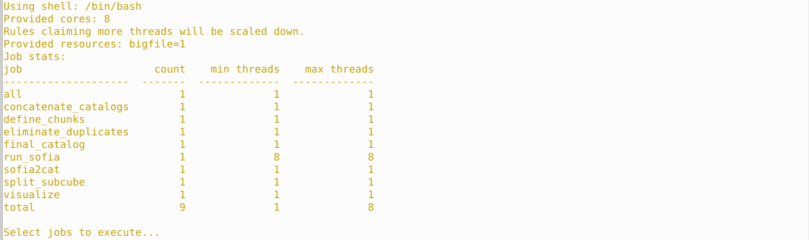
snakemake prompts a lot of the information in the terminal informing the user of what step is being executed and the percentage of completeness of the job. snakemake keeps its own logs within the directory .snakemake/logs/. For example, this is how one of the executions starts:

Using shell: /bin/bash
Provided cores: 32
Rules claiming more threads will be scaled down.
Provided resources: bigfile=1
Job stats:
job                     count    min threads    max threads
--------------------  -------  -------------  -------------
all                         1              1              1
concatenate_catalogs        1              1              1
final_catalog               1              1              1
run_sofia                  20             31             31
sofia2cat                  20              1              1
split_subcube              20              1              1
visualize                   1              1              1
total                      64              1             31

And then, each time a job is started, a summary of the job to be executed is shown. This gives you complete information of the state of the execution, and what and how is being executed at the moment. For example:

Finished job 107.
52 of 64 steps (81%) done
Select jobs to execute...

[Sat Jul 31 20:39:04 2021]
rule split_subcube:
    input: /mnt/sdc2-datacube/sky_full_v2.fits, results/plots/coord_subcubes.csv, results/plots/subcube_grid.png
    output: interim/subcubes/subcube_0.fits
    log: results/logs/split_subcube/subcube_0.log
    jobid: 4
    wildcards: idx=0
    resources: mem_mb=1741590, disk_mb=1741590, tmpdir=tmp, bigfile=1

Activating conda environment: /mnt/scratch/sdc2/jmoldon/hi-friends/.snakemake/conda/cf5c913dcb805c1721a2716441032e71

Apart from the snakemake logs, the terminal also displays information of the script being executed. By default, we save the outputs and messages of all steps in 6 subdirectories inside results/logs (see Output products for more details).

Configuration¶

The key parameters for the execution of the pipeline can be selected by editing the file config/config.yaml. This parameters file controls how the cube is gridded and how Sofia-2 is executed, among other options. The control parameters for Sofia-2 are directly controlled using the sofia par file. The template we use by default can be found in config/sofia_12.par. All the default configuration files can be found here: config.

Unit tests¶

To verify the outputs of the different steps of the workflow, we implemented a series of python unit tests based on the steps defined by the snakemake rules. The unit test contain simple examples of inputs and outputs of each rule, so when the particular rule in executed, their outputs are compared byte by byte to the expected output. The tests are passed only when all the output files match exactly the expected ones. These tests are useful to be confident that any changes introduced in the code during developement are producing the same results, preventing the developers to introduce bugs inadvertently.

As an example, we used myBinder to verify the scripts. The pipeline is installed automatically by myBinder. We executed the single command python -m pytest .tests/unit/ and obtained the following output:

jovyan@jupyter-hi-2dfriends-2dsdc2-2dhi-2dfriends-2dfsc1x4x2:~$ python -m pytest .tests/unit/
=================================================================== test session starts ===================================================================
platform linux -- Python 3.9.6, pytest-6.2.4, py-1.10.
rootdir: /home/jovyan
plugins: anyio-2.2.0
collected 6 items

.tests/unit/test_all.py .                                                                                                                           [ 16%]
.tests/unit/test_concatenate_catalogs.py .                                                                                                          [ 33%]
.tests/unit/test_define_chunks.py .                                                                                                                 [ 50%]
.tests/unit/test_final_catalog.py .                                                                                                                 [ 66%]
.tests/unit/test_run_sofia.py .                                                                                                                     [ 83%]
.tests/unit/test_sofia2cat.py .                                                                                                                     [100%]

============================================================== 6 passed in 206.24s (0:03:26) ==============================================================

This demonstrates that the workflow can be executed flawlessly in any platform, even with an unattended deployment as offered by myBinder.

Software managed and containerization¶

As explained above, the workflow is managed using snakemake, which means that all the dependencies are automatically created and organized by snakemake using conda. Each rule has its own conda environment file, which is installed in a local conda environment when the workflow starts. The environments are activated as required by the rules. This allows us to use the exact software versions for each step, without any conflict. We recommend that each rule uses its own small and individual environment, which is very convenient when maintaining or upgrading parts of the workflow. All the software used is available for download from Anaconda.

At the time of this release, the only conflict with this approach is that Sofia-2 has not yet created a conda package for version 2.3.0 that is compatible with Mac, so this approach will not work in MacOS. To facilitate correct usage from any platform, we have also containerized the workflow. We have used different container formats to encapsulate the workflow. In particular, we have definition files for Docker, Singularity and podman container formats. The Github repository contains the required files, and instructions to build and use the containers can be found in the installation instructions.

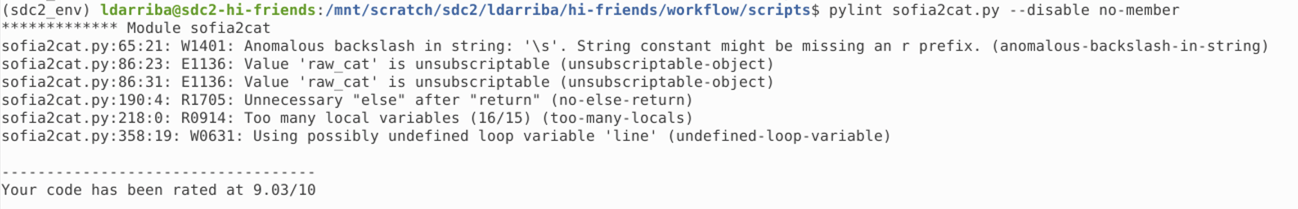
Check conformance to coding standards¶

Pylint is a Python static code analysis tool which looks for programming errors, helps enforcing a coding standard and looks for code smells (see Pylint documentation. It can be installed by running

pip install pylint

If you are using Python 3.6+, upgrade to get full support for your version:

pip install pylint --upgrade

For more information on Pylint installation see Pylint installation

We runned Pylint in our source code. Most of the code extrictly complies with python coding standards. The final pylint score of the code is:

Workflow Description¶

Workflow definition diagrams¶

The following diagram shows the rules executed by the workflow and their dependencies. Each rule is associated with the execution of either a python script, a jupyter notebook or a bash script.

rulegraph

The actual execution of the workflow requires some of the rules to be executed multiple times. In particular each subcube is processed sequentially. The next diagram shows the DAG of an example execution. The number of parallel jobs is variable, here we show the case of 9 subcubes, although for the full SDC2 cube we may use 36 or 49 subcubes.

dag

Each rule has associated input and output files. The following diagram shows the stage at which the relevant files are created or used.

filegraph

Workflow file structure¶

The workflow consists of a master Snakefile file (analogous to a Makefile for make), a series of conda environments, scripts and notebooks to be executed, and rules to manage the workflow tasks. The file organization of the workflow is the following:

workflow/
├── Snakefile
├── envs
│   ├── analysis.yml
│   ├── chunk_data.yml
│   ├── filter_catalog.yml
│   ├── process_data.yml
│   ├── snakemake.yml
│   └── xmatch_catalogs.yml
├── notebooks
│   └── sdc2_hi-friends.ipynb
├── rules
│   ├── chunk_data.smk
│   ├── concatenate_catalogs.smk
│   ├── run_sofia.smk
│   ├── summary.smk
│   └── visualize_products.smk
├── scripts
│   ├── define_chunks.py
│   ├── eliminate_duplicates.py
│   ├── filter_catalog.py
│   ├── run_sofia.py
│   ├── sofia2cat.py
│   └── split_subcube.py

Output products¶

All the outputs of the workflow are stored in results. This is the first level organization of the directories:

results/
├── catalogs
├── logs
├── notebooks
├── plots
└── sofia

In particular, each rule generates a log for the execution of the scripts. They are stored in results/logs. Each subdirectory contains individual logs for each executtion, as shown in this example:

logs/
├── concatenate
│   ├── concatenate_catalogs.log
│   ├── eliminate_duplicates.log
│   └── filter_catalog.log
├── define_chunks
│   └── define_chunks.log
├── run_sofia
│   ├── subcube_0.log
│   ├── subcube_1.log
│   ├── subcube_2.log
│   └── subcube_3.log
├── sofia2cat
│   ├── subcube_0.log
│   ├── subcube_1.log
│   ├── subcube_2.log
│   └── subcube_3.log
├── split_subcube
│   ├── subcube_0.log
│   ├── subcube_1.log
│   ├── subcube_2.log
│   └── subcube_3.log
└── visualize
    └── visualize.log

The individual fits files of the subcubes are stored in the directory interim because they may be large to store. The workflow can be setup to make them temporary files, so they are removed as soon as they are not needed anymore. After an execution, it is possible to maintain all the relevant outputs by keeping the results directory, while the interim directory, only containing fits files, can be safely removed if not explicitly needed.

interim/
└── subcubes
    ├── subcube_0.fits
    ├── subcube_1.fits
    ├── subcube_2.fits
    └── subcube_3.fits
    ...

Snakemake execution and diagrams¶

Additional files summarizing the execution of the workflow and the Snakemake rules are stored in summary. These are not generated by the main snakemake job, but need to be generated once the main job is finished by executing snakemake specifically for this purpose. The four commands to produce these additional plots are executed by the main script run.py.

summary/
├── dag.svg
├── filegraph.svg
├── report.html
└── rulegraph.svg

In particular, report.hml contains a description of the rules, including the provenance of each execution, as well as the statistics on execution times of each rule.

Interactive report showing the workflow structure:

When clicking in one of the nodes, full provenance is provided:

Statistics of the time required for each execution:

Workflow installation¶

This sections starts with the list of the main software used by the workflow, and a detailed list of all the dependencies required to execute it. Please, note that it is not needed to install these dependencies because the workflow will that automatically. The instructions below descripbe how to install the workflow locally (just by installing snakemake with conda, and snakemake will take care of all the rest). There are also instructions to use the containerized version of the workflow, using either docker, singularity or podman. The possible ways to deploy and use the workflow are:

Use conda to install snakemake through the environment.yml.
Build or download the docker container.
Build or download the singularity container.
Build or download the podman container.
Download the full tarball of the workflow (includes files of all software) in a Linux machine.
Open the Github repository in myBinder.

Dependencies¶

The main software dependencies used for the analysis are:

Sofia-2 (version 2.3.0) which is licensed under the GNU General Public License v3.0
Conda (version 4.9.2) which is released under the 3-clause BSD license
Snakemake (snakemake-minimal version 6.5.3) which is licensed under the MIT License
Spectral-cube(version 0.5.0) which is licensed under a BSD 3-Clause license
Astropy(version 4.2.1) which is licensed under a 3-clause BSD style license

The requirements of the HI-FRIENDS data challenge solution workflow are self-contained, and they will be retrieved and installed during execution using conda. To run the pipeline you only need to have snakemake installed. This can be obtained from the environment.yml file in the repository as explained in the installation instructions.

The workflow uses the following packages:

  - astropy=4.2.1
  - astropy=4.3.post1
  - astroquery=0.4.1
  - astroquery=0.4.3
  - dask=2021.3.1
  - gitpython=3.1.18
  - ipykernel=5.5.5
  - ipython=7.22.0
  - ipython=7.25.0
  - ipython=7.26.0
  - jinja2=3.0.1
  - jupyter=1.0.0
  - jupyterlab=3.0.16
  - jupyterlab_pygments=0.1.2
  - matplotlib=3.3.4
  - msgpack-python=1.0.2
  - networkx=2.6.1
  - numpy=1.20.1
  - numpy=1.20.3
  - pandas=1.2.2
  - pandas=1.2.5
  - pip=21.0.1
  - pygments=2.9.0
  - pygraphviz=1.7
  - pylint=2.9.6
  - pytest=6.2.4
  - python-wget=3.2
  - python=3.8.6
  - python=3.9.6
  - pyyaml=5.4.1
  - scipy=1.7.0
  - seaborn=0.11.1
  - snakemake-minimal=6.5.3
  - sofia-2=2.3.0
  - spectral-cube=0.5.0
  - wget=1.20.1

This list can also be found in all dependencies. The links where all the software can be downloaded is in all links.

It is not recommended to install them individually, because Snakemake will use conda internally to install the different environments included in this repository. This list is just for reference purposes.

Installation¶

To deploy this project, first you need to install conda, get the pipeline, and install snakemake.

1. Get conda¶

You don’t need to run this if you already have a working conda installation. If you don’t have conda follow the steps below to install it in the local directory conda-install. We will use the light-weight version miniconda. We also install mamba, which is a very fast dependency solver for conda.

 curl --output Miniconda.sh https://repo.anaconda.com/miniconda/Miniconda3-latest-Linux-x86_64.sh
 bash Miniconda.sh -b -p conda-install
 source conda-install/etc/profile.d/conda.sh
 conda install mamba --channel conda-forge --yes

2. Get the pipeline and install snakemake¶

git clone https://github.com/HI-FRIENDS-SDC2/hi-friends
cd hi-friends
mamba env create -f environment.yml
conda activate snakemake

Now you can execute the pipeline in different ways:

(a) Test workflow execution.

python run.py --check

(b) Execution of the workflow for Hi-Friends. You will need to modify the contents of config/config.yaml:

python run.py 

You can also run the unit tests to verify each individual step:

python -m pytest .tests/unit/

Deploy in containers¶

Docker¶

To run the workflow with the Docker container system you need to do the following steps:

Build the workflow image¶

Clone the respository from this github repository:

git clone https://github.com/HI-FRIENDS-SDC2/hi-friends.git

Change to the created directory:

cd hi-friends

Now build the image. For this we build and tag the image as hi-friends-wf:

docker build -t hi-friends-wf -f deploy.docker .

Run the workflow¶

Now we can run the container and then workflow:

docker run -it hi-friends-wf

Once inside the container:

(a) Test workflow execution.

python run.py --check

(b) Execution of the workflow for Hi-Friends. You will need to modify the contents of config/config.yaml:

python run.py 

Singularity¶

To run the workflow with singularity you can bild the image from our repository:

Build the image:¶

Clone the respository from this github repository:

git clone https://github.com/HI-FRIENDS-SDC2/hi-friends.git

Change to the created directory:

cd hi-friends

Build the Hi-Friends workflow image:

singularity build --fakeroot hi-friends-wf.sif deploy.singularity

Run the workflow¶

Once this is done, you can now launch the workflow as follows

singularity shell --cleanenv --bind $PWD hi-friends-wf.sif

And now, set the environment and activate it:

source /opt/conda/etc/profile.d/conda.sh
conda activate snakemake

and now, run the Hi-Friends workflow:

(a) Test workflow execution.

python run.py --check

(b) Execution of the workflow for Hi-Friends. You will need to modify the contents of config/config.yaml:

python run.py 

Podman¶

To run the workflow with podman you can build the image from our repository using our dockerfile:

Build the image:¶

Clone the respository from this github repository:

git clone https://github.com/HI-FRIENDS-SDC2/hi-friends.git

Change to the created directory:

cd hi-friends

Build the Hi-Friends workflow image:

podman build -t hi-friends-wf -f deploy.docker .

Run the workflow:

podman  run  -it hi-friends-wf

Run the workflow¶

Once inside the container:

(a) Test workflow execution.

python run.py --check

(b) Execution of the workflow for Hi-Friends. You will need to modify the contents of config/config.yaml:

python run.py 

Use tarball of the workflow¶

This solution only works with Linux environments. It has been tested in Ubuntu 20.04. First, download the tarball from Zenodo (link TBD).

You will need to have snakemake installed. You can install it with conda using this environment.yml. More information can be found in above.

Once you have the tarball and snakemake running, you can do:

tar xvfz my-workflow.tar.gz
conda activate snakemake
snakemake -n

Use myBinder¶

Simply follow this link. After some time, a virtual machine will be created with all the required software. You will start in a jupyter notebook ready to execute a check of the software. In general, myBinder is not thought to conduct heavy processing, so we recommend to use this option only for verification purposes.

Workflow execution¶

Preparation¶

This is a practical example following the instructions in section Workflow installation. Make sure you have snakemake available in your path. You may also be working inside one the proposed containers described in the section.

First we clone the repository.

$ git clone https://github.com/HI-FRIENDS-SDC2/hi-friends

This is what you will see.

Now, we access the newly created directory and install the dependencies:

$ cd hi-friends
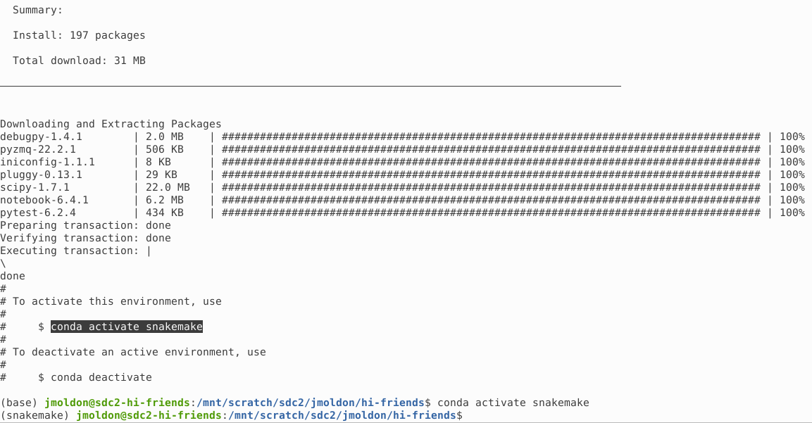
$ mamba env create -f environment.yml 

After a few minutes you will see the confirmation of the creation of the snakemake conda environment, which you can activate immediately:

Basic usage and verification of the workflow¶

You can check the basic usage of the execution script with:

$ python run.py -h

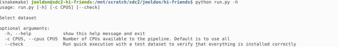
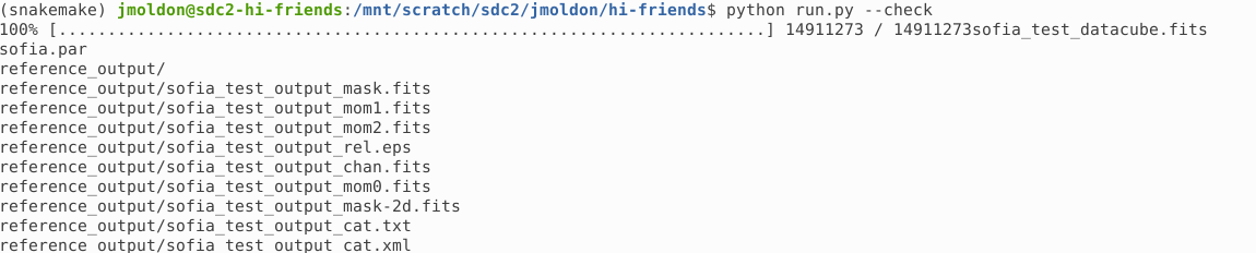
From here you can control how many CPUs to use, and you can enable the --check option, which runs the workflow in a small test dataset.

Using the --check option produces several stages. First, it automatically downloads a test dataset:

Second, snakemake is executed with specific parameters to quickly process this test datacube. Before executing the scripts, snakemake will create all the conda environments required for the execution. This operation may take a few minutes:

Third, snakemake will build a DAG to describe the execution order of the different steps, and execute them in parallel when possible:

Before each step is started, there is a summary of what will be executed and which conda environment will be used. Two examples at different stages:

After the pipeline is finished, snakemake is executed 3 more times to produce the workflow diagrams and an HTML report:

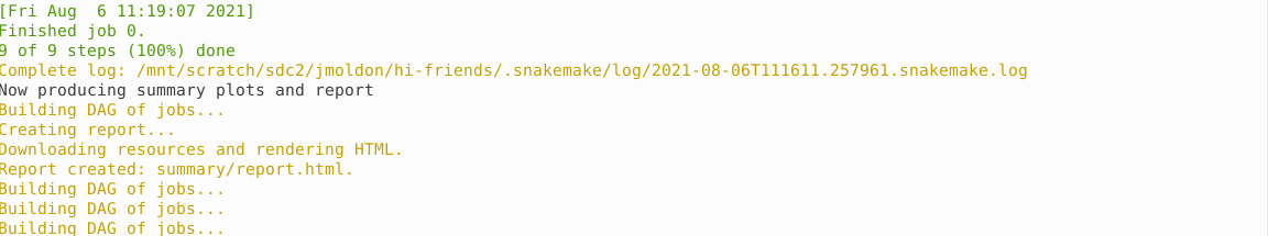
This is how your directory looks after the execution.

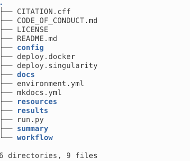
All the results are stored in results following the structure described in Output products. The interim directory contains subcube fits file, which can be removed to reduce used space.

Execution on a data cube¶

If you want to execute the workflow on your own data cube, you have to edit the config/config.yaml file. In particular, you must select the path of the datacube using the variable incube.

You may leave the other parameters as they are, although it is recommended that you adapt the sofia_param file with a Sofia parameters file that works best with your data.

Before re-executing the pipeline, you can clean all the previous products by removing directories interim and results. If you remove specific files from results, snakemake will only execute the required steps to generate the deleted files, but not the ones already existing.

$ rm -rf results/ interim/

You can modify the parameters file and execute run.py to run everything directly with python run.py. But you can also run snakemake with your preferred parameters. In particular, you can parse configuration parameters explicitly in the command line. Let’s see some examples:

Execution of the workflow using the configuration file as it is, with default parameters

snakemake -j32 --use-conda --conda-frontend mamba --default-resources tmpdir=tmp --resources bigfile=1

Execution specifying a different data cube:

snakemake -j32 --use-conda --conda-frontend mamba --default-resources tmpdir=tmp --resources bigfile=1 --config incube='/mnt/scratch/sdc2/data/development/sky_dec_v2.fits' 

You could define any of the parameters in the config.yaml file as needed. For example:

snakemake -j32 --use-conda subcube_id=[0,1,2,3] num_subcubes=16 pixel_overlap=4 --config incube='/mnt/scratch/sdc2/data/development/sky_dec_v2.fits' 

SDC2 HI-FRIENDS results¶

Our solution¶

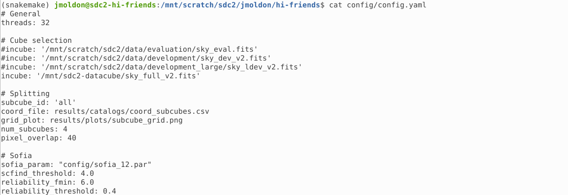
For our solution we used this configuration file:

# General
threads: 31

# Cube selection
#incube: '/mnt/scratch/sdc2/data/evaluation/sky_eval.fits'
#incube: '/mnt/scratch/sdc2/data/development/sky_dev_v2.fits'
#incube: '/mnt/scratch/sdc2/data/development_large/sky_ldev_v2.fits'
incube: '/mnt/sdc2-datacube/sky_full_v2.fits'

# Splitting
subcube_id: 'all'
coord_file: results/plots/coord_subcubes.csv
grid_plot: results/plots/subcube_grid.png
num_subcubes: 36
pixel_overlap: 40

# Sofia
sofia_param: "config/sofia_12.par"
scfind_threshold: 4.5
reliability_fmin: 5.0
reliability_threshold: 0.5

The 36 subcubes were gridded following this pattern: Example of subcube grid

The distribution of sources in the sky was: Detected catalog

We detected 22346 sources (once duplicates in the overlapping regions are removed).

This is the distribution of parameters in our catalog (blue), and how does it compare with the truth catalog of the large development cube (in grey), which covers a smaller area and therefore contains fewer sources. Please, note the different binning and the log scale used in some cases.

Parameters distribution

We then filtered the catalog to exclude sources that deviate significantly from the Wang et al. 2016 (2016MNRAS.460.2143W) correlation between HI size in kpc (\(D_HI\)) and HI mass in solar masses (\(M_HI\)). This is the resulting catalog:

Filtered by D-M correlation

These results will be uploaded to Zenodo.

Score¶

The solution presented by HI-FRIENDS obtained a total score of 13902.62 points in the challenge. This is the final leaderboard from the SDC2 website.

leaderboard

SDC2 Reproducibility award¶

In this section we provide links for earch item in the reproducibility award check list.

Reproducibility of the solution check list¶

Well-documented

[X] High-level description of what/who the software is for is available the HI-FRIENDS solution to the SDC2
[X] High-level description of what the software does is available software general description
[X] High-level description of how the software works is available workflow
[X] Documentation consists of clear, step-by-step instructions workflow installation execution methodology
[X] Documentation gives examples of what the user can see at each step e.g. screenshots or command-line excerpt execution
[X] Documentation uses monospace fonts for command-line inputs and outputs, source code fragments, function names, class names etc workflow installation execution developers
[X] Documentation is held under version control alongside the code repository

Easy to install

[X] Full instructions provided for building and installing any software workflow installation
[X] All dependencies are listed, along with web addresses, suitable versions, licences and whether they are mandatory or optional workflow installation. List of all required packages and their versions. Links to source code of each dependency including licenses when downloaded.
[X] All dependencies are available. Links to source code of each dependency including licenses when downloaded.
[X] Tests are provided to verify that the installation has succeeded. Unit tests, info unit tests
[X] A containerised package is available, containing the code together with all of the related configuration files, libraries, and dependencies required. Using e.g. Docker/Singularity docker, singularity

Easy to use

[X] A getting started guide is provided outlining a basic example of using the software e.g. a README file execution
[X] Instructions are provided for many basic use cases. execution on a data cube
[X] Reference guides are provided for all command-line, GUI and configuration options. basic usage execution on a data cube

Open licence

[X] Software has an open source licence e.g. GNU General Public License (GPL), BSD 3-Clause license
[X] License is stated in source code repository license
[X] Each source code file has a licence header source code

Have easily accessible source code

[X] Access to source code repository is available online repository
[X] Repository is hosted externally in a sustainable third-party repository e.g. SourceForge, LaunchPad, GitHub: Introduction to GitHub repository
[X] Documentation is provided for developers developers

Adhere to coding standards

[X] Source code is laid out and indented well source code
[X] Source code is commented source code
[X] There is no commented out code source code
[X] Source code is structured into modules or packages source code workflow file structure developers
[X] Source code uses sensible class, package and variable names source code
[X] Source code structure relates clearly to the architecture or design workflow file structure

Utilise tests

[X] Source code has unit tests. Unit tests, info unit tests
[X] Software recommends tools to check conformance to coding standards e.g. A ‘linter’ such as PyLint for Python. Pylint verification

Developers¶

define_chunks module¶

This script defines the coordintes of grid of subcubes

define_chunks.define_subcubes(steps, wcs, overlap, subcube_size_pix)¶

Return an array with the coordinates of the subcubes

Parameters

steps (int) – Steps to grid the cube.
wcs (class astropy.wcs) – wcs of the fits file
overlap (int) – Number of pixels overlaping between subcubes
subcube_size_pix (int) – Number of pixels of the side of the subcubes

Returns

coord_subcubes – Array with the coordinates of rthe subcubes

Return type

array

define_chunks.get_args()¶: This function parses and returns arguments passed in

define_chunks.main()¶: Chunk the data cube in several subcubes

define_chunks.plot_border(wcs, n_pix)¶

Plot boundaries of subcubes

Parameters

wcs (class astropy.wcs) – wcs of the fits file
n_pix (int) – Number of pixels of the cube side.

define_chunks.plot_grid(wcs, coord_subcubes, grid_plot, n_pix)¶

Plot grid of subcubes

Parameters

wcs (class astropy.wcs) – wcs of the fits file
coord_subcubes (array) – Array containing coordinates of subcubes.
grid_plot (str) – Path to save the grid plot
n_pix (int) – Number of pixels of the cube side.

define_chunks.plot_subcubes(coord_subcubes, l_s='-', color=None, l_w=1)¶

Plot subcubes

Parameters

coord_subcubes (int) – Steps to grid the cube.
l_s (str) – Line style. Defalult value is solid line
color (str) – Line color. Default value is no color.
l_w (float) – Line width. Default value is 1.

define_chunks.write_subcubes(steps, wcs, overlap, subcube_size_pix, coord_file)¶

Return coordinates of subcubes. Save file coord_file in the results folder containing the coordinates of the subcubes

Parameters

steps (int) – Steps to grid the cube.
wcs (class astropy.wcs) – wcs of the fits file
overlap (int) – Number of pixels overlaping between subcubes
subcube_size_pix (int) – Number of pixels of the side of the subcubes

Returns

Array containing coordinates of subcubes of the edges of the subcubes

Return type

coord_subcubes array

eliminate_duplicates module¶

This script removes duplicates and creates a catalog without duplicated sources

eliminate_duplicates.find_catalog_duplicates(ras, dec, freq)¶

Finds duplicates in the catalog

Parameters

ras (float) – Right ascension
dec (float) – Declination
freq (float) – Frequency

Returns

cond (Bool array) – array storing proximity criteria
idx (int array) – Index of the duplicated sources

eliminate_duplicates.get_args()¶: This function parses and returns arguments passed in

eliminate_duplicates.main()¶: Removes duplicates and creates a catalog without duplicated sources

eliminate_duplicates.mask_worse_duplicates(cond, idx, catalog_table)¶

Finds worse duplicates and masks them

Parameters

cond (Bool array) – array storing proximity criteria
idx (int array) – Index of the duplicated sources
catalog_table (astropy.Table) – table with detections

Returns

duplicates – array with True when source is duplicated

Return type

Bool array

eliminate_duplicates.read_coordinates_from_table(cat)¶

Reads coordinates from a table

Parameters

cat (astropy.Table) – table with coordinates

Returns

ras (float) – Right ascension
dec (float) – Declination
freq (float) – Frequency

eliminate_duplicates.read_ref_catalog(infile, name_list)¶

Reads the catalog with the variables from an input string

Parameters

infile (str) – Input file name
name_list (str) – List of varible names

Returns

catalog_table – table with the data

Return type

astropy.Table

filter_catalog module¶

This script filters the output catalog based on some conditions

filter_catalog.arcsec2kpc(redshift, theta)¶

Converts angular size to linear size given a redshift

Parameters

redshift (float) – redshift
theta (array of floats) – angular size in arcsec

Returns

distance_kpc – linear size in kpc

Return type

array of floats

filter_catalog.compute_d_m(cat)¶

Computes the Mass of HI and linear diameter of the galaxies in a catalog

Parameters: cat (pandas.DataFrame) – catalog of galaxies
Returns: cat – original catalog adding the columns log(M_HI) and log(D_HI_kpc)
Return type: pandas.DataFrame

filter_catalog.filter_md(df_md, uplim=0.45, downlim=- 0.15)¶

Removes items from a catalog based on distance from the Wang et al. 2016 2016MNRAS.460.2143W correlation. The values used are log DHI= (0.506±0.003) log MHI−(3.293±0.009)

Parameters

df_md (pandas DataFrame) – input catalog in pandas format
uplim (float) – Threshold distance to consider outliers in the top region
downlim (float) – Threshold distance to consider outliers in the bottom region

Returns

df_out – output catalog without the outliers

Return type

pandas DataFrame

filter_catalog.freq_to_vel(f0_hi=1420405751.786)¶

Convers line frequency to velocity in km/s

Parameters: f0_hi (float) – rest frequency of the spectral line
Returns: freq2vel – function to convert frequency in Hz to velocity
Return type: function

filter_catalog.get_args()¶: This function parses and returns arguments passed in

filter_catalog.main()¶: Gets an input catalog and filters the sources based on deviation from the D_HI M_HI correlation

run_sofia module¶

This script runs Sofia ***

run_sofia.eliminate_time(cat)¶

Eliminates timestamp from sofia catalog. Updates the file

Parameters: cat (str) – Path to sofia catalog

run_sofia.get_args()¶: This function parses and returns arguments passed in

run_sofia.is_tool(name)¶: Check whether name is on PATH and marked as executable.

run_sofia.main()¶: Runs Sofia if the output catalog does not exist

run_sofia.run_sofia(parfile, outname, datacube, results_path, scfind_threshold, reliability_fmin, reliability_threshold)¶

Only runs Sofia if the output catalog does not exist

Parameters

parfile (str) – File contanining parameters
outname (str) – Name of output file
datacube (str) – Path to data cube
results_path (str) – Path to save results
scfind_threshold (float) – Sofia parameter scfind_threshold
reliability_fmin (float) – Sofia parameter reliability_fmin
reliability_threshold (float) – Sofia parameter reliability_threshold

run_sofia.update_parfile(parfile, output_path, datacube, scfind_threshold, reliability_fmin, reliability_threshold)¶

Updates file with paramenters

Parameters

parfile (str) – File contanining sofia parameters
output_path (str) – Path of output file
datacube (str) – Path to datacube
outname (str) – Name of output file

Returns

updated_parfile – Path of file with updated parameters

Return type

str

sofia2cat module¶

This script converts sofia Catalog to the SDC2 catalog

sofia2cat.compute_inclination(bmaj, bmin)¶

Computes inclinaton See A7) in http://articles.adsabs.harvard.edu/pdf/1992MNRAS.258..334S Note p has been implemented as varp and q has been implemented as vaarq

Parameters

bmaj (float) – Major axis of ellipse fitted to the galaxy in arcsec
pix_x (float) – Minor axis of ellipse fitted to the galaxy in arcsec

Returns

np.degrees(np.arccos(cosi)) – Inclination in degrees

Return type

float

sofia2cat.convert_flux(flux, filename)¶

This assume that flux comes from SoFiA in Jy/beam and converts it to Jy * km/s base on the header

Parameters

flux (array of floats) – Flux in Jy/beam
filename (str) – Name of input file

Returns

flux_jy_hz – flux in Jy*Hz

Return type

array of floats

sofia2cat.convert_frequency_axis(filename, outname, velocity_req='radio')¶

Convert the frequency axis of a cube

Parameters

filename (str) – Name of input file
outname (str) – Name of output file
velocity_req (str) – velocity definition framework

sofia2cat.convert_units(raw_cat, fitsfile)¶

Convert units from raw catalog into fitsfile

Parameters

raw_cat (pandas DataFrame) – Raw catalog
fitsfile (string) – Path to fits file

Returns

ra_deg (array of floats) – Right ascension
dec_deg (array of floats) – Declination
pix2arcsec (float) – Conversion factor from pixel units to arcsec
pix2freq (float) – Conversion factor from channel to Hz

sofia2cat.find_fitsfile(parfile)¶

Searchs in the parfile the name of the fits file used

Parameters: parfile (str) – Parameters file
Returns: fitsfile – Path to fits file of processed data cube
Return type: str

sofia2cat.frequency_to_vel(freq, invert=False)¶

Convert frequency to velocity

Parameters

freq (float) – Frequency in Hz
invert (boolean) – If invert is false then returns velocity. If invert is true returns frequency.

Returns

ra_deg (array of floats) – Right ascension
dec_deg (array of floats) – Declination
pix2arcsec (float) – Conversion factor from pixel units to arcsec
pix2freq (float) – Conversion factor from channel to Hz

sofia2cat.get_args()¶: This function parses and returns arguments passed in

sofia2cat.main()¶: Converts sofia Catalog to the SDC2 catalog

sofia2cat.pix2coord(wcs, pix_x, pix_y)¶

Converts pixels to coordinates using WCS header info

Parameters

wcs (class astropy.wcs) – wcs of the fits file
pix_x (int) – Pixel number in X direction
pix_y (int) – Pixel number in Y direction

Returns

coord[0].ra.deg (float) – Right ascension in degrees
coord[0].dec.deg (float) – Declination in degrees

sofia2cat.process_catalog(raw_cat, fitsfile)¶

Process catalog

Parameters

raw_cat (pandas.DataFrame) – Raw catalog
fitsfile (str) – Path to fits file of processed data cube

Returns

processed_cat – Processed catalog

Return type

pandas.DataFrame

sofia2cat.read_sofia_header(filename)¶

Reads SOFIA header

Parameters: filename (str) – Input file name
Returns: head – Header of input file
Return type: str

sofia2cat.sofia2cat(catalog)¶

Runs sofia and returns the raw catalog filtered with galaxies that have: kinematic position angle greater than zero

Parameters: catalog (str) – Input file name
Returns: raw_cat_filtered – Raw catalog produced by sofia filtered by kinematic position angle greater than zero.
Return type: pandas DataFrame

split_subcube module¶

This script splits the cube in different subcubes according to a grid of subcubes

split_subcube.get_args()¶: This function parses and returns arguments passed in

split_subcube.main()¶: Splits the data cube in several subcubes

split_subcube.split_subcube(infile, coord_subcubes, idx)¶

Creates a fits file containing the coordinates x low x high y low and y high

Parameters

infile (str) – Input file name
coord_subcubes (array) – Array containing coordinates of subcubes
idx (int) – Index of subcube

Acknowledgments¶

Here we list the credits and acknowledgments for the members of the team.

This work used the SKA Regional Centre Prototype at IAA-CSIC, which is funded by the State Agency for Research of the Spanish MCIU through the “Center of Excellence Severo Ochoa” award to the Instituto de Astrofísica de Andalucía (SEV-2017-0709), the European Regional Development Funds (EQC2019-005707-P), by the Junta de Andalucía (SOMM17_5208_IAA), project RTI2018-096228-B-C31(MCIU/AEI/FEDER,UE) and PTA2018-015980-I(MCIU,CSIC).